JuliaTuesday

#TidyTuesday is a weekly data project aimed at the R ecosystem, aimed at developing skills in the tidyverse ecosystem. The Tidier.jl implementation aims to bring the tidyverse ecosystem to Julia!

I’ll be processing and visualising some of the #TidyTuesday data sets in Julia here!

2023/05/02: The Portal Project

The Portal Project is a long-term ecological research site studying the dynamics of desert rodents, plants, ants and weather in Arizona. This chart shows the number of Merriam’s kangaroo rats in 8 different plots. Plots 3, 15, 19, and 21 are exclosure plots whilst the rest are control plots. Merriam’s kangaroo rat has been surveyed the most often, especially in control plots.

Data: The Portal Project

Code

using Tidier
using UrlDownload
using DataFrames
using AlgebraOfGraphics, CairoMakie
using Colors

surveys = urldownload("https://raw.githubusercontent.com/rfordatascience/tidytuesday/master/data/2023/2023-05-02/surveys.csv") |> DataFrame ;
plots = urldownload("https://raw.githubusercontent.com/rfordatascience/tidytuesday/master/data/2023/2023-05-02/plots.csv") |> DataFrame ;

plot_data = @chain surveys begin
  @select(year, plot, species)
  @filter(species == "DM")
  @filter(plot in [3, 4, 11, 14, 15, 17, 19, 21])
  @group_by(year, plot)
  @summarise(n = nrow())
  @ungroup
  @left_join(plots)
end

plot_data[!,:plot] = [string(x) for x in plot_data[!,:plot]] 

xy = data(plot_data) * mapping(:year, :n, color=:treatment => "Treatment:", layout=:plot) * visual(Lines)

colors = ["exclosure" => colorant"#B23A48", "control" => colorant"#1F7A8C"]

with_theme(theme_ggplot2()) do
    draw(xy; legend=(position=:bottom, titleposition=:left, framevisible=false, padding=5),
         axis=(; ylabel="Number of Merriam's Kangaroo Rat observed", xlabel=""), facet=(; linkxaxes=:minimal), palettes = (color=colors, layout=[(2, 1), (2, 2), (3, 1), (3, 2), (4, 1), (4, 2), (1, 1), (1, 2)],))
end

2023/04/25: London Marathon

Since the first London Marathon in 1981, the number of people applying for a place in the race has drastically increased - especially in recent years. Over 450, 000 people applied for the 2020 race, which ended up taking place with only elite athletes due to Covid-19.

Data: Wikipedia via {LondonMarathon} R package

Code

using Tidier
using UrlDownload
using DataFrames
using AlgebraOfGraphics, CairoMakie

london_marathon = urldownload("https://raw.githubusercontent.com/rfordatascience/tidytuesday/master/data/2023/2023-04-25/london_marathon.csv") |> DataFrame ;

plot_data = @chain london_marathon begin
  @select(Year, Applicants)
  @filter(Applicants != "NA")
end

plot_data[!,:Applicants] = [parse(Int,x) for x in plot_data[!,:Applicants]] 

xy1 = data(plot_data) * mapping(:Year, :Applicants) * visual(BarPlot, color=:black, width=0.1)

xy2 = data(plot_data) * mapping(:Year, :Applicants) * visual(Scatter, color="#e00601")

with_theme(theme_ggplot2()) do
    draw(xy1 + xy2; axis=(; title="London Marathon", ylabel="Number of applicants", xlabel=""))
end

2023/04/18: Neolithic Founder Crops

Eight founder crops — emmer wheat, einkorn wheat, barley, lentil, pea, chickpea, bitter vetch, and flax — have long been thought to have been the bedrock of Neolithic economies. The world map below shows site locations considered in the Origins of Agriculture database, with sites highlighted based on their highest proportion of crops from different categories shown in the magnified versions on the right.

Data: The Neolithic Founder Crops in Southwest Asia: Research Compendium

Code

using Tidier
using UrlDownload
using DataFrames
using AlgebraOfGraphics, CairoMakie

founder_crops = urldownload("https://raw.githubusercontent.com/rfordatascience/tidytuesday/master/data/2023/2023-04-18/founder_crops.csv") |> DataFrame ;

plot_data = @chain founder_crops begin
  @filter(source == "ORIGINS")
  @filter(category != "NA")
  @select(category, site_name, prop)
  @group_by(site_name, category)
  @summarize(prop = mean(prop))
  @ungroup()
end

xy = data(plot_data) * mapping(:category, :prop) * visual(BoxPlot; color="#508080")

with_theme(theme_ggplot2()) do
    draw(xy; axis=(; title="Neolithic Founder Crops", ylabel="Proportion", xlabel=""))
end

2023/04/11: US Egg Production

The line chart shows the production (in millions) of cage-free organic eggs in the USA. The data used in this infographic is based on reports produced by the United States Department of Agriculture, which are published weekly or monthly.

Data: The Humane League Labs US Egg Production Dataset

Code

using Tidier
using UrlDownload
using DataFrames
using AlgebraOfGraphics, CairoMakie

production = urldownload("https://raw.githubusercontent.com/rfordatascience/tidytuesday/master/data/2023/2023-04-11/egg-production.csv") |> DataFrame ;

plot_data = @chain production begin
  @filter(prod_process == "cage-free (organic)")
  @mutate(n = n_eggs/1000000)
end

set_aog_theme!()

xy = data(plot_data) * mapping(:observed_month, :n) * visual(Lines)

draw(xy,
     axis=(ylabel="Cage-free organic eggs produced (millions)", xlabel=""))

2023/04/04: Premier League 2021-2022

Data: Kaggle

Code

using Tidier
using UrlDownload
using DataFrames
using AlgebraOfGraphics, CairoMakie
using LaTeXStrings
using Makie

soccer = urldownload("https://raw.githubusercontent.com/rfordatascience/tidytuesday/master/data/2023/2023-04-04/soccer21-22.csv") |> DataFrame ;

home_goals = @chain soccer begin
  @group_by(HomeTeam)
  @summarize(home_goals = sum(FTHG))
end

away_goals = @chain soccer begin
  @group_by(AwayTeam)
  @summarize(away_goals = sum(FTAG))
end

plot_data = @chain home_goals begin
  @left_join(away_goals, "HomeTeam" = "AwayTeam")
  @pivot_longer(plot_data, home_goals:away_goals)
  @mutate(text_vals = value+3)
end

set_aog_theme!()

xy1 = data(plot_data) * mapping(:HomeTeam,
                                :value,
                                layout=:variable => renamer("home_goals" => "Total Home Goals", "away_goals" => "Total Away Goals")) * visual(BarPlot, color=:black, width=0.1)

xy2 = data(plot_data) * mapping(:HomeTeam,
                                :value,
                                layout=:variable => renamer("home_goals" => "Total Home Goals", "away_goals" => "Total Away Goals")) * visual(Scatter)

draw(xy1 + xy2,
     axis=(ylabel="", xlabel="", xticklabelrotation=45.0),
     facet=(; linkxaxes=:minimal, linkyaxes=:minimal))

WARNING: using Makie.plots in module Main conflicts with an existing identifier.

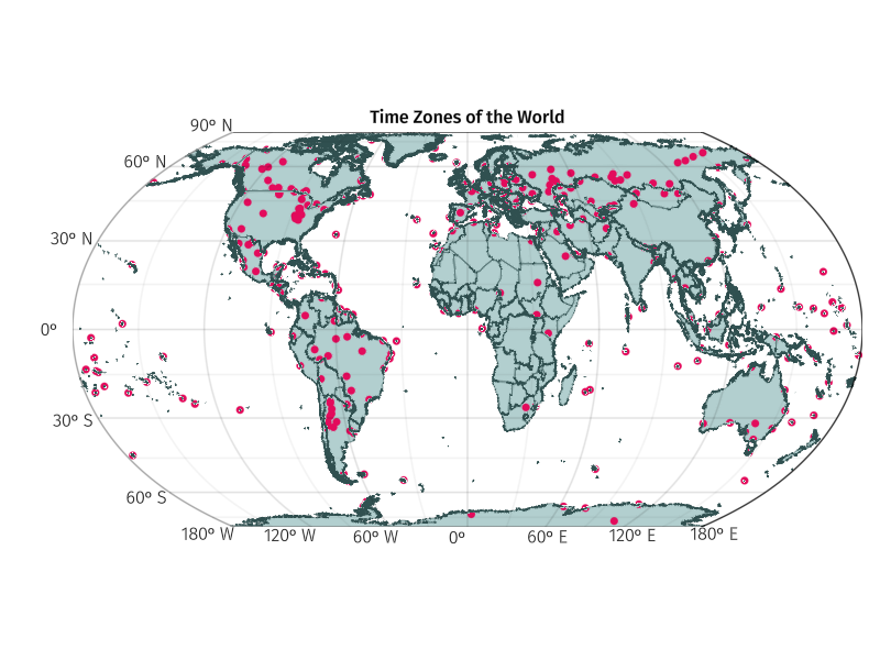
2023/03/28: Time Zones

Time zones tend to follow the boundaries between countries and their subdivisions instead of strictly following longitude. For every one-hour time, a point on the earth moves through 15 degrees of longitude. Each point relates to one of 337 time zones listed in the IANA time zone database. The colours show which time zones are in Africa, America, Antarctica, Asia, Atlantic, Australia, Europe, Indian, and Pacific zones.

Data: IANA tz database

Code

using UrlDownload
using DataFrames
using GeoMakie, CairoMakie
using Colors
using GLMakie

timezones = urldownload("https://raw.githubusercontent.com/rfordatascience/tidytuesday/master/data/2023/2023-03-28/timezones.csv") |> DataFrame ;

lons = -180:180
lats = -90:90
fig = Figure()
ax = GeoAxis(fig[1,1],
             title = "Time Zones of the World")

using GeoMakie.GeoJSON
countries_file = download("https://datahub.io/core/geo-countries/r/countries.geojson")
countries = GeoJSON.read(read(countries_file, String))

poly!(ax, countries;
    strokecolor = "#2F4F4F", strokewidth = 0.5,
    color="#b2cfcf"
)

slons = timezones[:, "longitude"]
slats = timezones[:, "latitude"]
scatter!(slons, slats, color= "#E30B5C", markersize=10)

fig

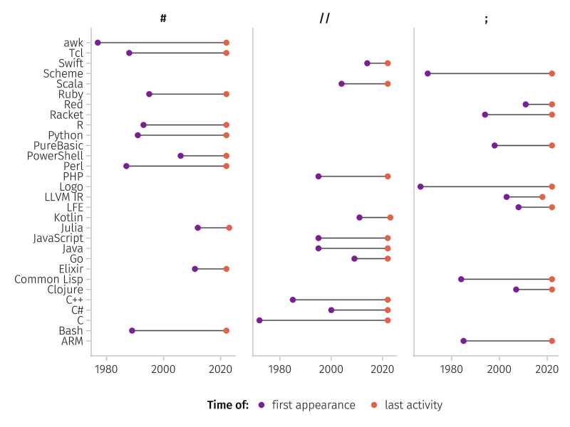
2023/03/21: Programming Languages

Of the 4,303 programming languages listed in the Programming Language DataBase, 205 use //, 101 use #, and 64 use ; to define which lines are comments. 3,831 languages do not have a comment token listed. The plots below show when a language first appeared, and when its last activity was.

Data: Programming Language DataBase

Code

using Tidier
using UrlDownload
using DataFrames
using AlgebraOfGraphics, CairoMakie
using Colors

languages = urldownload("https://raw.githubusercontent.com/rfordatascience/tidytuesday/master/data/2023/2023-03-21/languages.csv") |> DataFrame ;

plot_data = @chain languages begin
    @select(title, appeared, line_comment_token, last_activity, language_rank)
    @filter(line_comment_token in ["//", "#", ";"])
    @arrange(language_rank)
    @group_by(line_comment_token)
    @slice(1:10)
    @ungroup
    @pivot_longer(df_wide, appeared:last_activity)
    @filter(variable in ["appeared", "last_activity"])
end

set_aog_theme!()

xy1 = data(plot_data) * mapping(:value,
                               :title,
                               layout=:line_comment_token,
                               color=:variable => renamer("appeared" => "first appearance", "last_activity" => "last activity") => "Time of:")
layers1 = visual(Scatter)

xy2 = data(plot_data) * mapping(:value,
                                :title,
                                layout=:line_comment_token,
                                group=:title) * visual(Lines)


colors = [colorant"#791E94", colorant"#DE6449"]
draw(xy2 + layers1 * xy1,
     legend=(position=:bottom, titleposition=:left, framevisible=false, padding=5),
     axis=(ylabel="", xlabel="",  xticks=1980:20:2020),
     facet=(; linkxaxes=:minimal, linkyaxes=:minimal),
     palettes=(layout=[(1, 1), (1, 2), (1, 3)],
               color=colors))

2023/03/14: European Drug Development

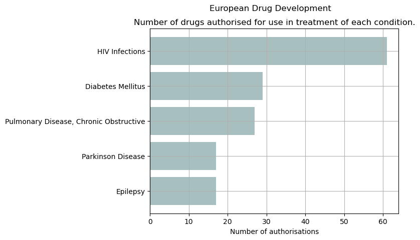
The European Medicines Agency (EMA) is the official regulator that directs drug development for both humans and animals, and decides whether to authorize marketing a new drug in Europe or not. Medicines for dogs are being authorised at a faster rate compared to other animals including pigs, cats, and chickens.

Data: European Medicines Agency

Code

using Tidier
using UrlDownload
using DataFrames
using PyPlot

drugs = urldownload("https://raw.githubusercontent.com/rfordatascience/tidytuesday/master/data/2023/2023-03-14/drugs.csv") |> DataFrame ;

plot_data = @chain drugs begin
    @select(therapeutic_area, authorisation_status)
    @filter(therapeutic_area in ["Epilepsy",
                                 "HIV Infections",
                                 "Parkinson Disease",
                                 "Diabetes Mellitus",
                                 "Pulmonary Disease, Chronic Obstructive"])
    @filter(authorisation_status == "authorised")
    @group_by(therapeutic_area)
    @summarize(n = nrow())
    @ungroup
    @arrange(n)
end

barh(plot_data[:, :therapeutic_area], plot_data[:, :n], color="#508080", align="center", alpha=0.5)
suptitle("European Drug Development");
title("Number of drugs authorised for use in treatment of each condition.");
xlabel("Number of authorisations")
grid("on")

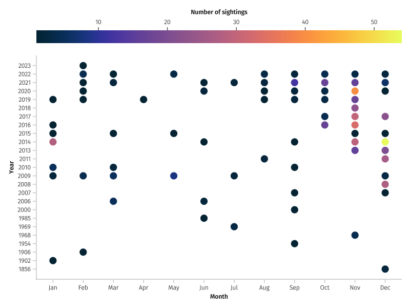
2023/03/07: Numbats

Numbats are small, distinctively-striped, insectivorous marsupials found in Australia. The species was once widespread across southern Australia, but is now restricted to several small colonies in Western Australia. They are therefore considered an endangered species. The calendar below shows thenumber of sightings of numbats per day between 2016 and 2022, using data from the Atlas of Living Australia. The full dataset includes data from 1856 to 2023 and, of the 805 observations, only 552 had dates recorded. Therefore the calendar may not reflect all numbat sightings.

Data: Atlas of Living Australia

Code

using Tidier
using UrlDownload
using DataFrames
using AlgebraOfGraphics
using CairoMakie

numbats = urldownload("https://raw.githubusercontent.com/rfordatascience/tidytuesday/master/data/2023/2023-03-07/numbats.csv") |> DataFrame ;
numbats = dropmissing(numbats, disallowmissing=true)

plot_data = @chain numbats begin
    @select(Month = month, Year = year)
    @filter(Month != "NA")
    @group_by(Month, Year)
    @summarize(n = nrow())
    @ungroup
    @arrange(Month)
end

set_aog_theme!()
update_theme!(fontsize=12, markersize=20)

numbats_plot = data(plot_data) * mapping(:Month => renamer("Jan" => "Jan", "Feb" => "Feb", "Mar" => "Mar", "Apr" => "Apr", "May" => "May", "Jun" => "Jun", "Jul" => "Jul", "Aug" => "Aug", "Sep" => "Sep", "Oct" => "Oct", "Nov" => "Nov", "Dec" => "Dec"), :Year, color = :n => "Number of sightings") * visual(colormap=:thermal)
AlgebraOfGraphics.draw(numbats_plot, colorbar=(position=:top, size=25))

2023/02/28: African Language Sentiment

Over 100,000 tweets in 14 different African languages were analysed to uncover the sentiment of the text. Sentiment analysis was performed and each tweet was labelled as either positive, negative, or neutral. Nigerian pidgin is particularly notable for its very few neutral tweets.

Data: AfriSenti

Code

using Tidier
using UrlDownload
using VegaLite

afrisenti = urldownload("https://raw.githubusercontent.com/rfordatascience/tidytuesday/master/data/2023/2023-02-28/afrisenti.csv") |> DataFrame ;

plot_data = @chain afrisenti begin
    @select(language_iso_code, label)
    @group_by(language_iso_code, label)
    @summarize(n = nrow())
    @ungroup
end ;

plot_data |>
@vlplot(
    :bar,
    x={:n, axis={title="Number of tweets"}},
    y={:language_iso_code, axis={title=""}},
    color={
        :label,
        scale={
            domain=["positive","neutral","negative"],
            range=["#407e6e","#a4a4a4","#374A67"]
        }
    }
)